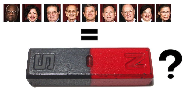
I just read an interesting new physics paper that’s posted up on the arxiv. It’s called the Statistical mechanics of the US Supreme Court, and it attempts to understand how Supreme Court judges influence each other when voting, using techniques from the physics of magnetism.
What’s the goal of this study?
Let’s say you looked up the numbers on how each supreme court judge has voted over a decade. Using this data, can you work out how much the judges influence each other? Are they voting independently, or do the votes of their peers influence their decision?
Now, you might think this is pretty easy. After all, we all know that US politics is dominated by ideological affiliations, so the strongest factor deciding a judge’s vote is probably whether they’re a liberal or a conservative. The 9 Supreme Court judges are split into a right and a left, with a few swing votes, and so you might expect that the most likely outcome is a 5-4 vote.
Turns out that this isn’t the case. Here’s a plot of the breakup of supreme court votes from 1946 to 2005. Surprisingly, unanimous decisions are twice as likely as a 5-4 split.
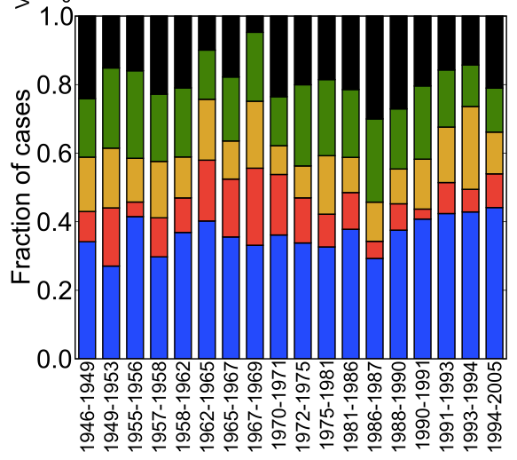
The goal of this paper is to take this data and come up with a model of how the supreme court justices influence each other.
Why is this hard to do?
The first thing the authors did with the data was to look at how correlated each judge’s vote is with every other judge. They focused on data from 1994 – 2005 (the second Rehnquist court). Here’s a figure, from their paper, that shows these correlations.
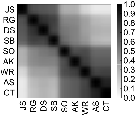
A positive correlation between two judges means that they are likely to vote for the same outcome. Surprisingly, even though the supreme court has strong ideological differences, there are no negative correlations between judges. This means that no two judges consistently vote against each other. However, some judges are more likely to agree than others. You can see this in the two blocks of high correlation in the figure above (top left and bottom right). The judges are arranged from political left (on the left) to political right (on the right). Unsurprisingly, the left and the right form two distinct voting blocks. That means judges on the left are more likely to agree with each other, and judges on the right are more likely to agree with each other. No surprise there.
But the physicists behind this paper didn’t just wanted to know how judge votes were correlated. They wanted to understand how the judges actually influenced each other. At the heart of the issue is the difference between correlation and influence.
I asked my friend John Barton to explain this. John is a physicist who specializes in the techniques used in this paper.
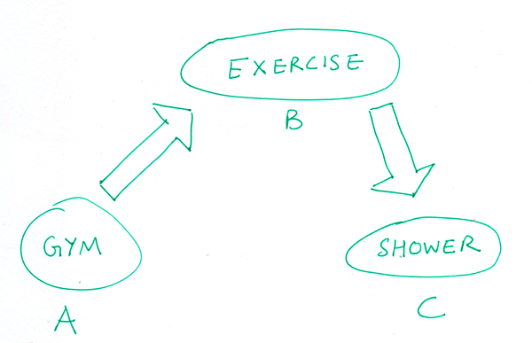
It sounds rather complicated, but at the heart of it all they’re really trying to do is sort out “influence” from “correlation.” For example (silly example, I’ve heard better ones but I can’t remember them right now so just making this one up!), consider three variables: A : “X is at the gym,” B : “X is exercising,” and C : “X takes a shower.” All these variables will be correlated, but A and C only influence each other indirectly. I’m only more likely to take a shower after going to the gym if I exercised while I was there. So in this simple picture I would see interactions between A and B, and between B and C, but not between A and C.
The key insight of this paper was to go from the list of correlations between judge votes, and actually work out the direct influences that the judges have on each other.
But there’s a hitch. It turns out that there are infinitely many ways in which judges can influence each other, that all give rise to the same voting behavior. So how do you figure out which set of interactions is the best one to choose?
So what does this have to do with magnets?
The solution has its roots in the physics of magnetism. Here’s how it works. Imagine you had a magnet. If you zoom in to this magnet with the right kind of microscope, you’d see tiny little microscopic magnets – each of which can either align with or against each other. These micro-magnets (or spins, which is what physicists call them) can flip their directions, and they can influence each other – every micro-magnet tries to get the other ones to align with itself. Some micro-magnets are more influential than others, and they can convince many others to flip in their direction.


Turns out, this magnet model maps nicely to the supreme court problem. Just as the micro-magnets influence each other’s orientation, and arrive at an emergent magnetization, the supreme court judges can influence each other’s votes, and from their deliberations emerges a final vote. The researchers used the same tool (maximum entropy) to identify the influences between the judges as one uses to work out the interactions between spins in a magnet.
The key insight is to imagine that supreme court justices influencing each other are like magnetic spins interacting with each other.

How well does the model work?
The central question for any model is, of course, does it explain the data? Turns out this model does a pretty good job.
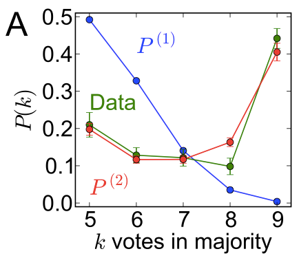
The green curve in the plot shows how often the supreme court has a certain vote outcome. For example, their votes result in a 5-4 majority 20% of the time, and 6-3 majority 12% of the time, and so on, until a 9-0 unanimous decision about 40% of the time.
Now, if each judge was voting independently of their colleagues, you’d expect to see the blue curve. You can see that it utterly fails to reproduce the data. Judges talk.
Finally, if each judge influenced the others in just the way predicted by the magnet model from above, you get the red curve. As you can see, it lines up pretty nicely with the green, and reproduces the fact that a 9-0 unanimous decision is twice as likely as a 5-4 majority.
What did they learn from this?
The researchers found the set of interactions between supreme court judges that best reproduces the data. What did that teach them?
Here’s one example. They found that a positive vote by the most conservative judge, Clarence Thomas, increases the odds of a positive vote by the most liberal judge, John Paul Stevens, by 10%. This goes against ideological reasoning. But take another conservative judge, Antonin Scalia, who has a very similar voting record to Clarence Thomas. In comparison to Thomas, a positive vote by Scalia actually pulls Stevens in the opposite direction, decreasing his odds of a positive vote by 30%.
In other words, the researchers were able to unmask the interactions hiding in the correlation data. They could work out the subtle ways in which the judges can bias each other’s decisions.
They went on to show, in agreement with our intuition, that the least influential supreme court judges from 1994-2005 were the ones at the ideological extremes (Scalia and Thomas). According to their results, the most influential judges in this period were Sandra Day O’Connor and Anthony Kennedy, who are typically seen as ‘swing votes’.
In summary, this method applies the tools of statistical physics to understand how a very, very influential group of people comes to a decision. In addition to reproducing the main features of the voting data, it also uncovers subtle biases in decision making. While this method won’t tell you how the court will vote on a given case, it will tell you about how they influence each other, on average.
Personally, I think it’s fascinating that we can understand how very smart humans make complex decisions using much of the same physics that describes a fridge magnet.
References
Statistical mechanics of the US Supreme Court. Edward D. Lee, Chase P. Broedersz, William Bialek. arxiv link. (Submitted on 20 June 2013)
If you’re interested in more work along these lines, here’s an afterword by John:
William Bialek is a maximum entropy/inverse Ising guru, and has applied this kind of analysis in several different areas (most famously to model the firing statistics of networks of neurons). For a couple more applications of this same technique you might want to check out this paper by Bialek and company, which really helped to kick off this approach for looking at neural networks, or this paper from my current group, which looked at fitness of HIV viruses.
