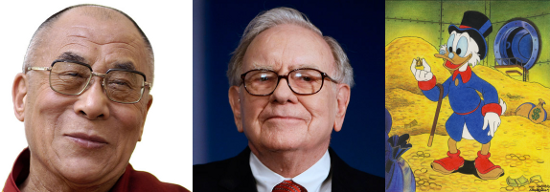
What the Dalai Lama can teach us about temperatures below absolute zero

3heads_550px
What can these three teach us about temperature?

There’s been a lot of buzz lately in the science blogosphere about a recent experiment where physicists created a gas of quantum particles with a negative temperature – negative as in, below absolute zero. This is pretty strange, because absolute zero is supposed to be that temperature at which all atomic motion ceases, where atoms that normally jiggle about freeze in their places, and come to a complete standstill. Presumably, this is as cold as cold can be. Can anything possibly be colder than this?

Here’s the short answer. It is possible to create negative temperatures. It was actually first done in 1951. But it’s not what it sounds like – these temperatures aren’t colder than absolute zero. For instance, you can’t keep cooling something down to make its temperature drop below absolute zero. In fact, as I’ll try to explain, objects at a negative temperature actually behave as if they’re HOTTER than objects that are at any positive temperature.

To understand this, we first need to know what physicists mean by temperature. You may remember from high school physics or chemistry that temperature measures the average kinetic energy of motion of particles. When you heat a substance, you’re speeding up its molecules, and when you cool it down, you’re slowing the molecules down.

This definition really made sense to me when I could see it for myself, so here is a simulation where you can play around with gas molecules. Go switch on the heater, and then turn up or down the heat, and see what happens.

So far, so good. But physicists realized that this definition of temperature doesn’t always work, because there are more types of energy than kinetic energy of motion. There are even situations where an object has an energy, but there isn’t really anything moving around in the conventional sense, like the magnetic spins in a magnet, or the ones and zeros on your hard disk. These are essentially quantum systems, where it doesn’t really make sense to talk about stuff moving, but you can still write down how much energy it has. It became clear that physics needed a more fundamental definition of temperature, that would make room for these possibilities.

Here’s the new definition that they came up with. Temperature measures the willingness of an object to give up energy. Actually, I lied. This isn’t how they really define temperature, because physicists speak math, not english. They define it as \frac{1}{T} = \frac{dS}{dE} which says, in words, that the temperature is inversely proportional to the slope of the entropy vs. energy curve.

Now, if you don’t speak math, I’m going to let you in on a little secret. You don’t need to know any math or physics to understand how temperature works. You can use a surprisingly accurate analogy. I first heard this analogy as an undergraduate, in an excellent thermal physics textbook by Daniel Schroeder.

isolated commune

Picture a world where people are constantly exchanging money to attain happiness. This is probably not that hard for you to imagine. But there’s a small twist.

The people in this society have agreed that they will work to maximize happiness – not just their own happiness, but the total happiness in the society. This has surprising consequences. For example, there might be some people who get very happy when they earn a little money. We could call them greedy. Other people don’t really care much about money – they become a little happier when they earn some money, and a little sadder when they lose it. These people are generous – if they’re playing by the rules of the game, they ought to give money to greedy people, to raise the overall happiness of society.

So why am I inventing this socialist utopia with rampant income redistribution? It’s because this is closely analogous to the physics of heat (as Steven Colbert put it, reality has a well know liberal bias).

Here’s the analogy. The socialist commune is what physicists call an isolated system. The people are the objects in this system. The money that they exchange is really energy – a quantity whose total amount is conserved, but that is constantly being exchanged. Happiness is entropy – just as the society wants to maximize happiness, physical systems are driven to maximize their total entropy. And finally, generosity is temperature, the willingness of people (i.e. objects) to give up money (i.e. energy).

This is a lot to swallow, so here’s a handy dictionary that lets you translate from our analogy to real physics:

\mbox{money} \leftrightarrow \mbox{energy}

\mbox{happiness} \leftrightarrow \mbox{entropy}

\mbox{generosity} \leftrightarrow \mbox{temperature}

By looking up this dictionary, everything that we say about our commune is translated into a statement about physics.

Now, imagine that our society consists of people like Warren Buffett. Initially, when they’re poor, getting money makes them very happy. But as they get wealthier, the same amount of money doesn’t make them nearly as happy. If you plot the happiness of these Buffett-like people versus their wealth, it would look something like this.
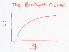
buffett curve 1

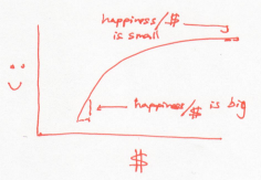
buffett curve 2
For the Buffetts, happiness per dollar (greediness) falls as you earn more money

In this world, every dollar earns you less happiness than the last one. So to raise the overall happiness, a rich Buffett should give money to a poor Buffett. This is a world where people become more generous as they acquire money. Or a system whose temperature rises as it gains energy.

The Buffett curve describes normal particles that we know and love, whose temperatures rise as you heat them. These are the jiggling atoms in solids, liquids, or gases.

Now, instead, consider a world of people who are misers, like Uncle Scrooge. Every dollar they earn makes them more happy than the previous dollar did.
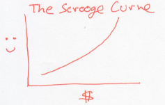
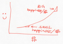
scrooge curve 1

Happiness per dollar (greediness) rises with more money.
For Scrooges, happiness per dollar (greediness) rises with more money

Unlike the Buffetts, if a rich Scrooge gives a dollar to a poor Scrooge, this would lower the overall happiness of Scrooges. In other words,  the Scrooges generosity decreases as they acquire more money. Using our dictionary, this is a system whose temperature drops as it gains energy.

Chew on that last thought for a moment. Could you really have an object that gets colder as you give it energy?

This really happens, when you have a bunch of particles that attract each other. Stars are held together by gravity, and they behave in just this way. As a star loses energy, its temperature rises. Give a star energy, and you’re actually cooling it down. Black holes also behave in this odd way – the more energy you feed them, the bigger they get, and yet, the colder they get.

And if that wasn’t counter-intuitive enough for you, here’s another scenario. Picture a world of people who have attained enlightenment – they actually become happier when they lose money.
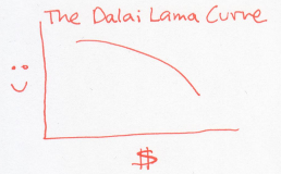
dalai lama curve

In this example, every dollar that the Dalai Lama receives actually makes him sadder. The natural tendency, then, is to give away all his money to whoever is willing to take it. This odd, inverted curve, is exactly the situation that results in negative temperatures – just relabel happiness to entropy and money to energy (mathematically, the curve has negative slope, so it must have negative temperature).

What happens when a negative temperature object meets a positive temperature object? To find out, imagine that the Dalai Lama meets Warren Buffett.

2heads_500px

Paradoxically, the Dalai Lama will give his money away to the billionaire, because losing money will make the Dalai Lama happier, and gaining money will make Waren Buffett just a teeny bit happier. In this strange exchange, the net happiness goes up. Using our dictionary, energy flows from a negative temperature object to an object that is at any positive temperature!

This might sound like something dreamt up by an over-zealous theorist. But there are real materials where the entropy versus energy curve looks like the Dalai Lama’s happiness versus money curve, i.e. where the temperature is negative.

To get here, you first need to engineer a system that has an upper limit to its energy. This is a very rare thing – normal, everyday stuff that we interact with has kinetic energy of motion, and there is no upper bound to how much kinetic energy it can have.

Systems with an upper bound in energy don’t want to be in that highest energy state. Just as the Dalai Lama is not happy with a lot of money, these systems have low entropy in (i.e. low probability of being in) their high energy state. You have to experimentally ‘trick’ the system into getting here.

This was first done in an ingenious experiment by Purcell and Pound in 1951, where they managed to trick the spins of nuclei in a crystal of Lithium Fluoride into entering just such an unlikely high energy state. In that experiment, they maintained a negative temperature for a few minutes. Since then, negative temperatures have been realized in many experiments, and most recently established in a completely different realm, of ultracold atoms of a quantum gas trapped in a laser.

From black holes to quantum gases, this analogy shows us that temperature is a lot more subtle than what we measure on a thermometer.

References

Here’s a very charming blog post that explains temperature using Leprechauns and Laser Beams.

The money and happiness analogy is not my own, but borrowed from the marvelous physics textbook Thermal Physics by Daniel Schroeder.

Statistical Mechanics by Pathria and Beale has a nice discussion on how magnetic systems can realize negative temperatures (via Tim Prisk).

John Baez’s blog on negative temperature and the entropy of stars.

The physics of that ‘kickalicious’ kick

Last Friday, the New York Times ran a cover page story about Håvard Rugland, a Norwegian man who scored an NFL tryout for the Jets, based on a youtube video called Kickalicious that has picked up nearly 2 million views. In this video, he pulls of a series of very impressive football kicks, with seemingly inhuman accuracy.

Personally, I found the last trick the hardest to believe (3:42 onwards). I wasn’t alone in my skepticism. Here’s what the New York Times had to say about it:

The most eye-popping trick is saved for last. Rugland punts one ball high into the air and then quickly kicks a second ball off a tee. The balls collide in midair.

“That last kick, it took about eight tries,” Rugland said. “The basketball kick, I wanted it to go straight in, but it kept hitting the rim. That actually took a while. That could have been like 40 tries.”

Rugland is so accurate on so many difficult kicks that his video almost seems too good to be true. It brings to mind doctored videos featuring other athletes, like one of the Los Angeles Lakers star Kobe Bryant leaping over a speeding Aston Martin (Bryant never would have risked his knees). But Rugland insisted his video was real. He said that NRK, Norway’s public broadcasting network, reviewed the raw videos and concluded they were legitimate.

So, inspired by Rhett Allain’s blog posts, I decided to try my hand at analyzing this video with physics.

Try Science

I downloaded a clip of the last trick, and opened it up in Tracker, an open source physics toolkit for video analysis.

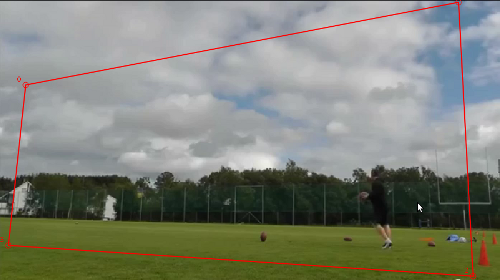
The first problem is that there is a pretty massive perspective distortion in the video. The video camera is pretty close to Rugland, and it’s inconveniently positioned at an angle. Fortunately, tracker has a handy tool that lets you morph the video to correct for this perspective distortion. (Here’s Rhett explaining how to use it).

Here’s the video before correcting for perspective:

before perspective

And here it is afterwards:

after perspective

Before correction, the ‘parallel lines’ of the treetops, fence and the turf aren’t really parallel – they converge to a point. After the correction, they seem more or less parallel.

The next step is to track the two footballs. I made a video of what the trick shot looks like when you do this. The first ball is in red, the second in light blue, and the green dots show you the center of mass of the two balls (The center of mass is the midpoint of the line that connect the two balls).

So far, so good. Now, on to the physics. If these trickshots are legitimate, they should come close to obeying the laws of projectile motion. In particular, if you plot the height of each projectile over time, you should get a parabola described by the equation

\mbox{height} = v_{0y}t + \frac{1}{2} g t^2

Here t is time, v_{0y} is the vertical launch speed of the ball at time zero, and g is the one number that everyone remembers from a physics course  – the acceleration due to gravity, which is -9.81 \frac{m}{s^2}.

If you haven’t seen this equation before, all you need to know is that it represents a parabola, and that you can test whether an object is really in free fall by fitting this equation to the data. What’s more, you can try and extract the known acceleration due to gravity.

To do this, take the coefficient of the t^2 term in that equation, and multiply it by two. You should recover the acceleration due to gravity g = -9.81 \frac{m}{s^2}.

Does this work for the trick shot? The first thing I need to do is set the scale in the video, so we can convert on-screen distances to real life distances. To do this, I assumed that Rugland is about 6 feet tall (1.8 meters), and am guessing this is accurate to about 20% or so. So I don’t expect any result I get to be more accurate than this.

Update: Rugland told me on twitter that he is 1.9 meters tall, so this guess is well within 10 percent.

football to scale

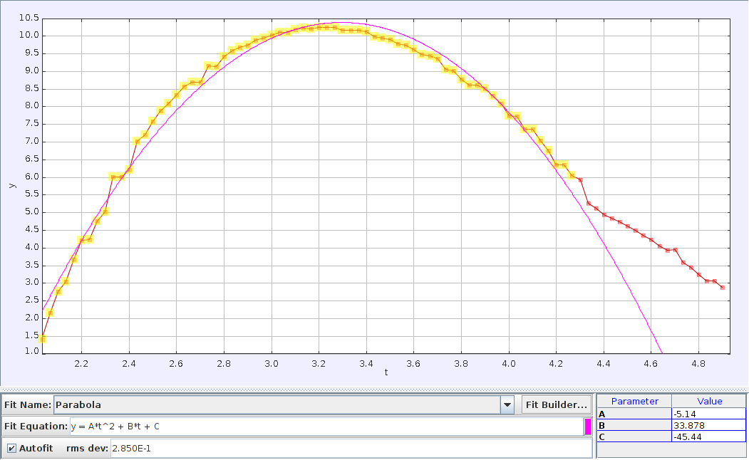
Now, to the plots! First up is the plot of the height of the first football (vertical axis), plotted versus time (horizontal axis).

ball 1 parabola

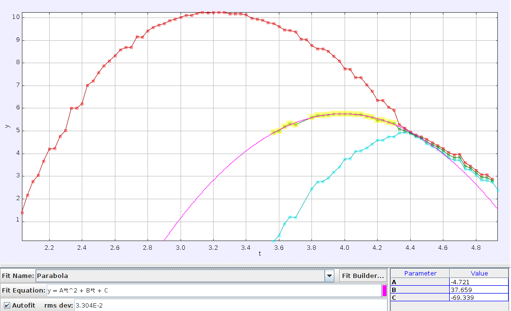
Tracker fits this curve to a parabola, and you can see that the trajectory of the ball (red line) is quite close to the parabola (pink line). I only used data from BEFORE the collision (in yellow) to fit the curve. After the collision, you wouldn’t expect it to stay on the same parabolic path. The curve fit is surprisingly good, considering that there’s definitely some wind resistance, lens distortion, and remaining issues with perspective.

Do we recover the value of gravitational acceleration (g = -9.81 \frac{m}{s^2})  from this curve? If I take the parameter A from the curve fit and double it, I get g = -10.28 \frac{m}{s^2}. That’s just 5 percent away from the actual value, which is far more accurate than we have any reason to expect.

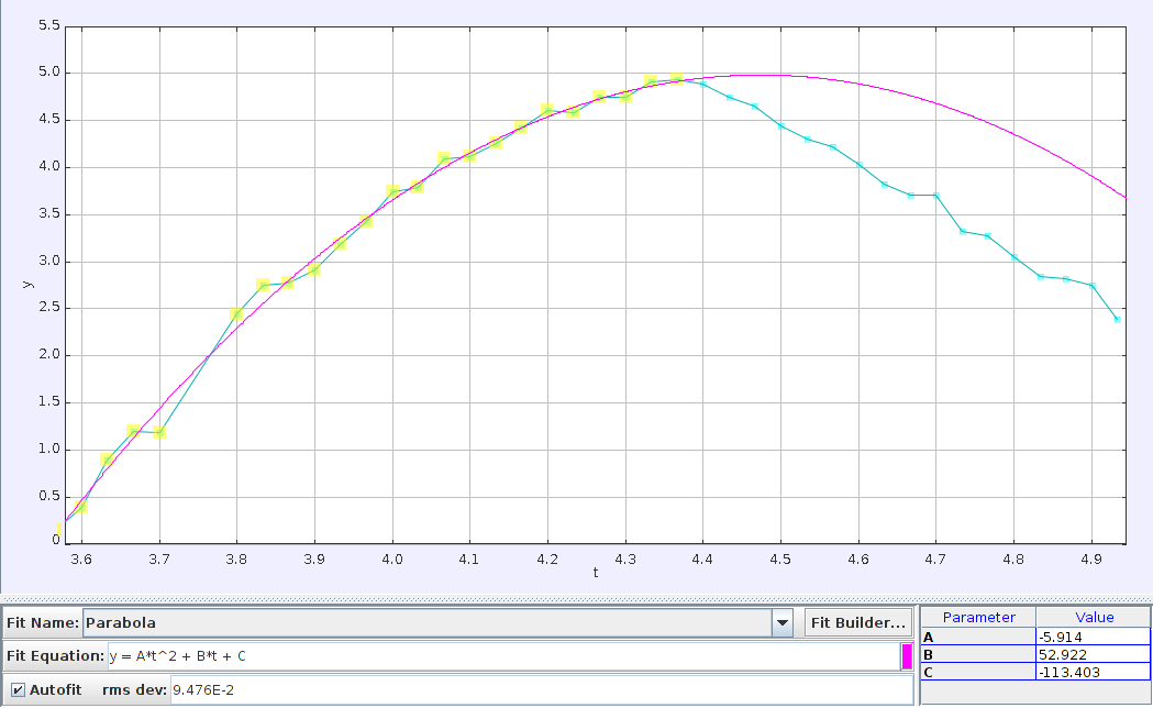
How about the second ball? Here it is the curve for its height vs. time:

ball 2 parabola

Same trick as before. I used Tracker to fit the second ball’s curve to a parabola (considering only data up till the collision). Then, I just multiply the parameter A times two to get the acceleration due to gravity. This time I get  g = -11.84 \frac{m}{s^2}, which is about 17 percent away from the known value. Again, not too shabby. (The pink line is what you would expect if you extrapolated the balls trajectory to after the collision. In reality, of course, it smacked into the other ball and made a significant course adjustment).

Before we take the next step, I need to introduce a new concept. Imagine that you have a firework in your hand, and you light it and throw it into the air. It begins to trace out a nice, neat parabola. What happens after it explodes? Suddenly, instead of one particle you have dozens, and everything looks like a mess. There is a way out of this mess, and it involves the concept of center of mass.

What physics tells us is that after the firecracker explodes, if we considered the average position of all the little exploded chunks of firecracker, then that average position (the center of mass) will still trace out a parabola. It doesn’t matter if it’s a tiny firecracker or a spectacular fireworks display, all the internal forces of the explosion will cancel out, and the center of mass will trace out a boring, old parabola.

What does this have to do with the two footballs? Well, you can think of a collision as an explosion in reverse. (Update: Added in that link, via Ed Yong on Twitter.) The same idea holds – the center of mass of the two footballs isn’t bothered by the collision. Now, of course, the forces in the collision will dramatically alter the trajectory of each football – they’re bumping into each other, after all. BUT, if you consider the two footballs as one extended system, then these bumps are internal forces, and they cancel each other out (Heck yeah, Newton’s 3rd Law). The upshot is that if we plot the center of mass of the two footballs, we should see a parabola that isn’t really affected by the collision.

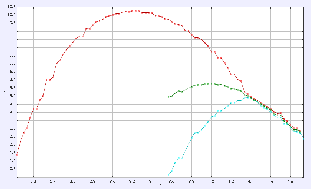
Here’s a plot of both balls (red and blue), and the center of mass of the two balls (in green).

both balls plus CM
Fireworks in reverse?

After the collision, the two footballs converge to their center of mass. (This is what physicists call a highly inelastic collision, because the two particles basically stick to each other. It means that the energy of motion, kinetic energy, isn’t being conserved, probably because the balls start to spin wildly and are therefore bleeding energy in to the rotational motion).

Now, I’m going to take the curve traced by the center of mass (in green) and fit the data points before the collision to a parabola. If this collision is really obeying the laws of physics, then the center of mass shouldn’t care about the collision, and the green curve after the collision should stay on the same path.

Here’s what I get:

2 balls plus center of mass curve fit

The pink curve is the predicted trajectory, based on extrapolating the center of mass motion from before the collision. The green curve (sandwiched between the red and blue) is the real data. It’s not dead on, but it’s no too far either.

One possible reason for the discrepancy is that after the collision, the footballs might move sideways to some extent (i.e. perpendicular to the plane of the camera). This would make the center of mass calculation inaccurate after the collision. Also, at this point the balls are at their furthest from the camera, so the perspective correction might not be so great at this distance.

I’m going to go ahead and say that this video is for real. No one would fake a video while also bothering to preserve the center of mass trajectory!

Kudos to you Håvard Rugland, and I hope you kick some ass in that NFL tryout!


Nerdy footnote:

When you have a hammer, it’s fun to hammer things. For no particular reason, here are a few more numbers that we can infer from the data. Rugland kicked Ball 1 at an angle of about 64 degrees at a speed of about 32 mph. About 1.5 seconds later, and 1.5 meters ahead, he kicked Ball 2 at an angle of 40 degrees and at a speed of about 38 mph. It’s a pretty cool testament to Rugland’s abilities that he’s basically able to solve a physics problem in his head that would give most undergrads a severe headache!

For more gratuitous (and hopefully fun) physics, check out my post on the physics of leaping lemurs, where I solve for the launch speed and launch angle of a sifaka lemur.

What does randomness look like?

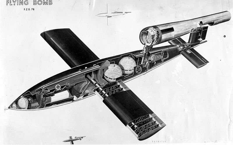
800px-V-1_cutaway

On 13 June 1944, a week after the allied invasion of Normandy, a loud buzzing sound rattled through the skies of battle-worn London. The source of the sound was a newly developed German instrument of war, the V-1 flying bomb. A precursor to the cruise missile, the V-1 was a self-propelled flying bomb, guided using gyroscopes, and powered by a simple pulse jet engine that gulped air and ignited fuel 50 times a second. This high frequency pulsing gave the bomb its characteristic sound, earning them the nickname buzzbombs.

From June to October 1944, the Germans launched 9,521 buzzbombs from the coasts of France and the Netherlands, of which 2,419 reached their targets in London. The British worried about the accuracy of these aerial drones. Were they falling haphazardly over the city, or were they hitting their intended targets? Had the Germans really worked out how to make an accurately targeting self-guided bomb?

Fortunately, they were scrupulous in maintaining a bomb census, that tracked the place and time of nearly every bomb that was dropped on London during World War II. With this data, they could statistically ask whether the bombs were falling randomly over London, or whether they were targeted. This was a math question with very real consequences.

Imagine, for a moment, that you are working for the British intelligence, and you’re tasked with solving this problem. Someone hands you a piece of paper with a cloud of points on it, and your job is to figure out if the pattern is random.

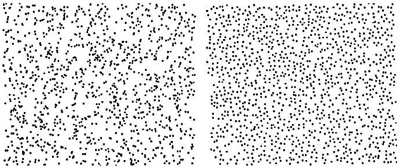
Let’s make this more concrete. Here are two patterns, from Steven Pinker’s book, The Better Angels of our Nature. One of the patterns is randomly generated. The other imitates a pattern from nature. Can you tell which is which?

pinker-glow-worms-and-stars-plot

Thought about it?

Here is Pinker’s explanation. Continue reading What does randomness look like?

What is the true measure of a storm?

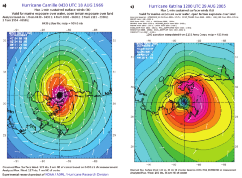
Satellite images of Hurricanes Camille (left) and Katrina (right). Source: NOAA

As Hurricane Katrina surged towards New Orleans, people faced the unthinkable prospect of abandoning their homes and finding shelter. Worst affected were some of the city’s most vulnerable citizens, the poor and the elderly, parents with young children, people without cars, and people living in flood-prone areas. Among those who stayed back, many were old enough to remember Hurricane Camille, a category 5 storm that devastated the region in 1969. Many homes were spared from flooding then, so it stood to reason that they should hold up to Katrina, also a category 5 storm that was demoted to a category 3 by the time it hit land. Sadly, they were mistaken, as the category rating of the hurricane was not the best measure of the raw destructive power of the storm.

The Saffir-Simpson rating system

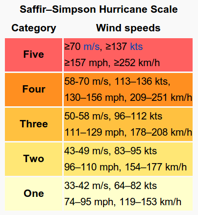
In the western hemisphere, hurricanes are all rated on the Saffir-Simpson scale, an empirical measure of storm intensity devised in 1971 by civil-engineer Herbert Saffir and meteorologist Bob Simpson. To compute a storm’s category rating, you have to measure the highest speed sustained by a gust of wind for an entire minute. The wind’s speed is measured at a height of 10 meters  because wind speeds increase as you climb higher, and it is here that they do the most damage. Based on how large this maximum speed is, a storm is assigned to one of five different categories.

Source: Wikipedia

The problem with this number is that it only captures one aspect of a storm’s intensity – the highest speed that it can sustain. Not only is it tricky to measure this peak speed, but different organizations may come to different conclusions about it, depending on their coverage of the wind data. This number doesn’t tell you anything about the size of the storm, nor about how the wind-speeds are distributed overall.

Consider a tale of two storms – the first is fierce but more contained, whereas the second is larger, and though it has lower peak wind speed, these wind speeds are spread over a larger area. The SS scale would give the first storm a higher score, even though the latter may be more destructive. Based on the rating, people might have expected Katrina to be about as destructive as Camille.

A tale of two storms. On the left is Hurricane Camille, a category 5 storm that struck the Gulf Coast in 1969. On the right is Katrina, a category 3 as it hit the same coast in 2005. Warmer colors correspond to higher wind speeds. Although peak wind speed was higher in Camille, high winds spread over a larger region in Katrina, leading to more widespread destruction. Source: NOAA

A rip in the wind tapestry

So how can one take the true measure of a storm? Storms are dangerous because of the energy carried in the moving air. Unless you live in a windy city, or drive your car at high speed on an interstate, you probably don’t think of air as something that carries much energy. But in a storm, strong winds ram into stationary objects, like trees, buildings, or the surface of the ocean, and impart some of their energy of motion. Some structures can safely absorb this energy, while others will give way.

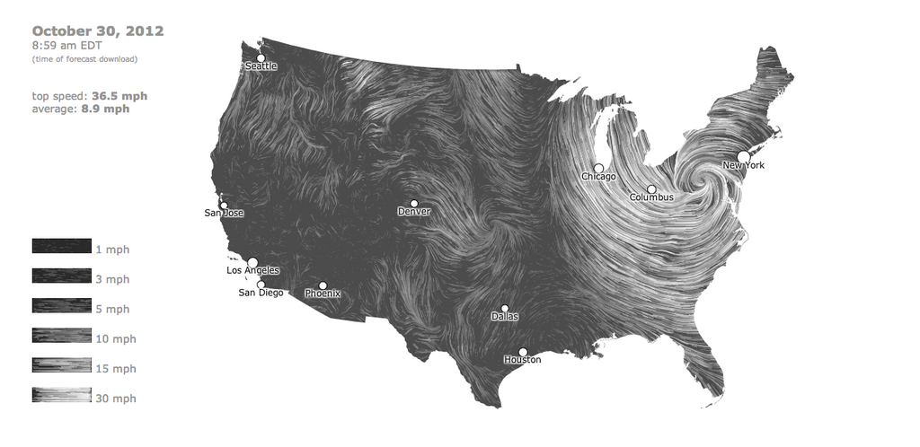
The Wind Map for the morning after Hurricane Sandy made landfall in the US

As Hurricane Sandy made its way through the US, many turned to this incredible real-time wind map to get a larger picture of the storm. I watched Sandy as it made landfall, and was mesmerized by the unexpected beauty that underlies this destructive force. On most days, if you look at the wind map, you’ll find a seamless tapestry made up of delicate threads and broader, sweeping strokes. The wind weaves its way through the central mountains, and brushes through the plains in wide swathes, leaving trails like a comb pulled through the hair of an unruly child. It’s a flow that is sculpted by geography and powered by the ebb and flow of weather systems. Visualizing this flow is like watching a globe-sized zen garden rearrange itself, tended not by any individuals, but by the blind, mathematical laws of fluid dynamics.

On this day, as Hurricane Sandy pummeled through the north-eastern US states, the winds started to pick up outside my window in New Jersey, and the trees swayed violently as the gusts grew stronger. On the wind map, there seemed to be a giant bald spot, a rip in the wind tapestry where from where threads had started to fray.
Continue reading What is the true measure of a storm?

Can we build a more efficient airplane? Not really, says physics.

Update (13 October):  I emailed David MacKay to get his opinion on some of the critical comments responding to this blog post. David is a physicist at Cambridge University, author of the book ‘Sustainable Energy – Without the Hot Air’, and is the chief scientific adviser to the UK Department of Energy and Climate Change. You can read his response in the comments below. There’s also a interesting discussion of this post over at hacker news.

Boeing recently launched a new line of aircraft, the 787 Dreamliner, that they claim uses 20% less fuel than existing, similarly sized planes.

How did they pull off this sizeable bump in fuel efficiency? And can you always build a more fuel-efficient aircraft? Imagine a hypothetical news story, where a rival company came up with a new type of airplane that used half the fuel of its current day counterparts. Should you believe their claim?

More generally, do the laws of physics impose any limits on the efficiency of flight? The answer, it turns out, is yes.

Jet Man, by Ben Heine

There’s something about flying that doesn’t sit well with us. If we never saw a bird fly, it may never have occurred to us to build flying machines of our own.

Here’s where I think this sense of unease comes from. It takes stuff to support stuff. Everyday objects fall unless other things get in their way. Take the floor away, and you’ll plummet to your doom – the air below your feet isn’t going to do much for you. We move through air so effortlessly, that we barely notice it’s there. So what keeps a plane up? There doesn’t seem to be enough ‘stuff’ there to hold up a bird, let alone a Boeing aircraft weighing up to 500,000 pounds. To put that last number in context, its more than the weight of an adult blue whale!

Why is it that planes fly and whales typically don’t? The answer is easy to state, but its consequences are rather surprising. Planes fly by throwing air down. That’s basically it. It’s an important point, so I’ll say it again. Planes fly by throwing air down.

As a plane hurtles through the air, it carves out a tube of air, much of which is deflected downwards by the wings. Throw down enough air fast enough, and you can stay afloat, just as the downwards thrust of a rocket pushes it up. The key is that you have to throw down a lot of air (like a glider or an albatross), or throw it down really fast (like a helicopter or a hummingbird).

A physicist’s two-step guide to flight (it’s simple, really!)

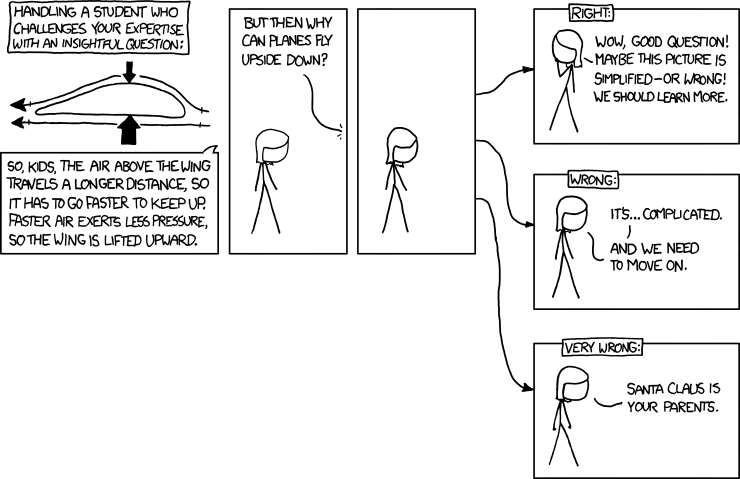
Let’s make this idea more quantitative. Following David MacKay’s wonderful book on Sustainable Energy, I’m going to build a toy model of flight. A good model should give you a lot of bang for the buck. The means being able to predict relevant quantities about the real world while making a minimum of assumptions.

Toy models gone wrong. By Randall Munroe at XKCD.

Step 1: Sweep out a tube of air

As a plane moves, it carves out a tube of air. This air was stationary, minding its own business, until the airplane rammed into it. This costs energy, for the same reason your car’s fuel efficiency drops when you speed up on the highway. Your car has to shove air out of its way.

Exactly how much energy does this cost? You might remember from high school physics that it takes an amount of energy equal to 1/2 m v^2 to bring stuff with mass m up to a speed v.

In our case, we have

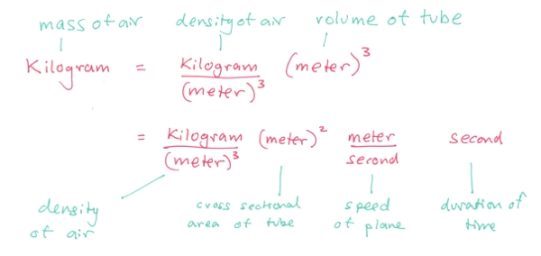
There’s still this mysterious factor of the mass of the air tube. To work this out, we can use a favorite trick in the toolbox of a physicist – unit cancellation. We can re-write the humble kilogram as a seemingly complicated product of terms.

What we’ve done here is to express an unknown mass of air in terms of other quantities that we do know. Each of these terms makes sense. Air that’s more dense will weigh more. A fatter plane (larger cross-sectional area) sweeps out more air, as does a faster plane. We’ve arrived at a meaningful result, just by playing around with units. In the words of Randall Munroe, unit cancellation is weird.

Put these two ideas together and here’s what you find:

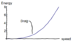
Here’s a graph of what that looks like.

If you’re with me so far, we just found that for a plane to plow through air, it has to expend an amount of energy proportional to the speed of the plane to third power. (The extra factor of v comes from the fact that faster planes sweep out a larger mass of air.) If you want to go twice as fast, you need to work 8 times as hard to shove air out of your way.

We’ve arrived at a general rule about the physics of drag. This holds true for a car on the highway, or for a swimmer or cyclist in a race. It’s why drag racing cars get only about 0.05 miles to a gallon! If we want to reduce overall energy consumption by cars, one option is to lower the speed limits on highways.

What does this mean for our toy plane? It would seem that the slower the plane, the higher its efficiency. So are airplane speed limits also in order? Absolutely not! To see why, read on to the second half the story..

Step 2: Throw the air down

In order to fly, a plane must throw air downwards. This generates the lift that a plane needs to stay up. It turns out that slower planes have to throw air harder to stay afloat. That’s why slow moving hummingbirds and pigeons have to flap their wings frenetically. It’s also why planes extend flaps while landing – they’re not throwing the air fast enough, so they compensate by throwing more of it.

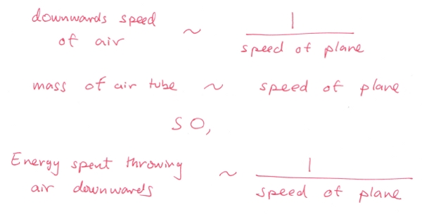
More precisely, for a plane to stay afloat, the speed of the air jettisoned downwards must be inversely proportional to the speed of the plane. (You can take my word for this, although if you want to see where it comes from, take a look at David MacKay’s book.)

So we can now work out the second part of the puzzle. How much energy does it take to throw air down? As before, this is given by

Just as we did in the first step, let’s express things in terms of the speed of the plane.

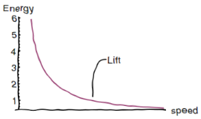
In words, the energy spent in generating lift is inversely proportional to the speed of the plane. Here’s what this looks like on a graph.

You can see from the plot that, as far as lift is concerned, slower flight is less efficient than faster flight, because you have to work harder in throwing air downwards.

There’s a lot to chew on here. To summarize, we’ve discovered that in making a machine fly, you have to spend energy (really fuel) in two ways.

  1. Drag: You need to spend fuel to push air away. This keeps you from slowing down.
  2. Lift: You need to spend fuel to throw air down. This is what keeps the plane afloat.

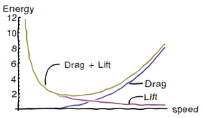
The total fuel consumption is the sum of these two parts.

If you fly too fast, you’ll spend too much fuel on drag (think of a drag racer or an F-16). Fly too slow, and you’ll have to spend too much fuel on generating lift, like a hummingbird furiously flapping its wings, powered by high calorie nectar. However, at the bottom of this curve there is a happy minimum, an ideal speed that resolves this tradeoff. This is the speed at which a plane is most efficient with its fuel. Be it through the ingenuity of aircraft engineers, or the ruthless efficiency of natural selection,  airplanes and birds are often fine-tuned to be as energy efficient as possible.

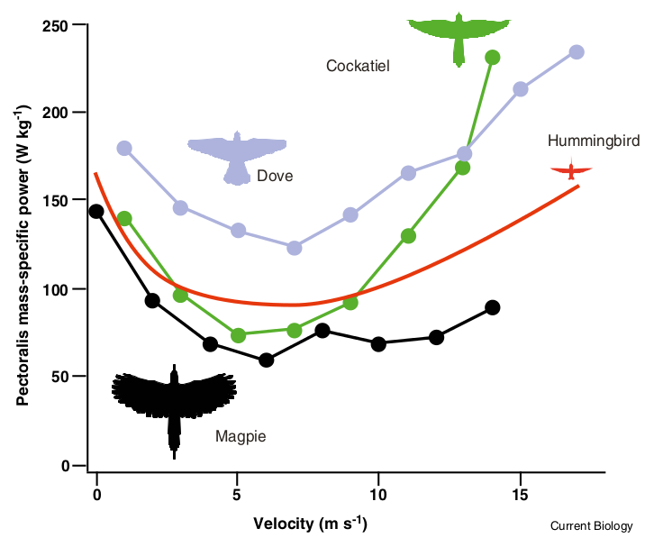
Here’s a plot of experimental data of the power consumption of different birds, as their flight speed varies.

You can see that it matches the qualitative predictions of the toy model.

But we can do more than this, and actually extract quantitative predictions from the model. An undergraduate schooled in calculus should be able to work out that special optimal speed at which energy consumption is a minimum. David MacKay plugs in the numbers in  his book, and finds that the optimal speed of an albatross is about 32 mph, and for a Boeing 747 is about 540 mph. Both these numbers are remarkably close to the real values. Albatrosses fly at about 30-55 mph, and the cruise speed of a Boeing 747 is about 567 mph. 

That’s a lot of mileage from a toy model!

And so our model teaches us that flying machines should never have speed limits. Whether made of metal or meat, every plane has an ideal speed. If you stray from this value, you have to pay for it in fuel cost. Slowing a car down may improve your mileage, but for a plane, the mileage actually gets worse.

And with this physicsy interlude into the world of albatrosses, hummingbirds, and jet planes, we come back to the question of the fuel efficiency of Boeing’s new aircraft.

You can actually use the model to work out the fuel efficiency of a plane. What you find is that it really just depends on a few factors: the shape and surface of the plane, and the efficiency of its engine. And of these factors, the engine efficiency plays the biggest role. So we would predict that engine efficiency, followed by improvements in body design might drive Boeing’s fuel savings.

This agrees with Boeing’s own assessment.

New engines from General Electric and Rolls-Royce are used on the 787. Advances in engine technology are the biggest contributor to overall fuel efficiency improvements.

New technologies and processes have been developed to help Boeing and its supplier partners achieve the efficiency gains. For example, manufacturing a one-piece fuselage section has eliminated 1,500 aluminum sheets and 40,000 – 50,000 fasteners.

Try as we like, we can’t squeeze a lot of improvement out of airplanes. Engines are already remarkably efficient, and you certainly can’t shrink the size of a plane by much, as economy class passengers can well attest. New manufacturing techniques could cut the amount of drag on the plane’s surface, but these improvements would only raise fuel efficiency by about 10%.

To quote David Mackay,

The only way to make a plane consume fuel more efficiently is to put it on the ground and stop it. Planes have been fantastically optimized, and there is no prospect of significant improvements in plane efficiency.

A 10% improvement? Yes, possible. A doubling of efficiency? I’d eat my complimentary socks.

References

I based this blog post on material I learnt from David MacKay’s fantastically clear book, Sustainable Energy without the Hot Air. It’s available online for free, and is highly recommended for anybody looking to use numbers to understand energy.

David MacKay (2009). Sustainable Energy – Without the Hot Air UIT Cambridge Ltd

I used this tip to make those XKCD style plots.

Milk, meat and blood: how diet drives natural selection in the Maasai

This post is a little different from the usual fare at this blog, as I am discussing a paper on which I’m a co-author. My collaborators and I just put up a paper in the open-access journal PLOS ONE. We analyzed genetic data from members of the Maasai tribe in Kenya and detected genes related to lactase persistence and cholesterol regulation that are under positive selection.

The Maasai and their Diet

Maasai tribe member drinking blood. Image credit: Rita Willaert

The Maasai are a pastoralist tribe living in Kenya and Northern Tanzania. Their traditional diet consists almost entirely of milk, meat, and blood. Two thirds of their calories come from fat, and they consume 600 – 2000 mg of cholesterol  a day. To put that number in perspective, the American Heart Association recommends consuming under 300 mg of cholesterol a day. In spite of a high fat, high cholesterol diet, the Maasai have low rates of diseases typically associated with such diets. They tend to have low blood pressure, their overall cholesterol levels are low, they have low incidences of cholesterol gallstones, as well as low rates of coronary artery diseases such as atherosclerosis.

Even more remarkable are the results of a 1971 study by Taylor and Ho. Two groups of Maasai were fed a controlled diet for 8 weeks. One group – the control group – was given food rich in calories. The other group had the same diet, but with an additional 2 grams of cholesterol per day. Both diets contained small amounts of a radioactive tracer (carbon 14). (You’d never get approval for a study like this today, and for good reason.) By monitoring blood and fecal samples, the scientists discovered that the two groups had basically identical levels of total cholesterol in their blood. In spite of consuming a large dose of cholesterol, these individuals had the same cholesterol levels as the control group.

Here is how the authors concluded their study:

This led us to believe, but without direct proof, that the Masai have some basically different genetic traits that result in their having superior biologic mechanisms for protection from hypercholesteremia

Motivated by these results, we set out to identify genes under selection in the Maasai as a result of these unusual dietary pressures. We scanned the genome looking for genetic signatures of natural selection at work.

The Data

Our data comes from the International HapMap Project, a collaborative experimental effort to study the genetic diversity in humans. The HapMap Project has collected DNA from groups of people from genetically diverse human populations with ancestry in Africa, Asia and Europe. Their anonymized data is publicly available for free. One of the HapMap populations is a group of Maasai from Kinyawa, Kenya  (n=156), and this is the population that we focus on.

DNA sequences on a part of Chromosome 7 from two random individuals, with the differences shown in red.

HapMap does not sequence full genomes, as this would have been prohibitively expensive at the time of data collection. Instead, they employ a shortcut. If you take my DNA sequence and line it up against yours, the two sequences will be about 99.9% similar. But every once in a thousand letters, or so, there will be a difference. You may have an A where I have a C. The HapMap group measures the DNA sequence at these very locations, where humans are known to vary from each other. In essence, they’re sampling the genome, looking only at sites where we expect to see variation. In the jargon of the field, this method is called looking for Single Nucleotide Polymorphisms, or SNPs (pronounced snips).

Hunting for signatures of selection in genetic data

Once you have the data, what can you do with it? We wanted to detect signs of natural selection. The basic idea behind detecting selection in genomic data is quite simple, and it has to do with sex. Every sperm or egg cell that you produce contains a single genome, which is formed by shuffling together the two sets of genomes that you inherited from your parents. Viewed this way, the role of sex is to shuffle together the genomes in a population into new combinations. If you compare the DNA sequences of a group of people, you will see signs of this shuffling.

The effect of sex is to shuffle genomes, in a process known as genetic recombination.

Now lets add natural selection to the mix. What happens if an individual is born with a new mutation that benefits their survival? Over time, you’d expect to see this mutation rise in frequency. Descendants of this individual will be over-represented in the population, as the fraction of people with this beneficial mutation goes up. In essence, the fingerprint of such selection is a reduction of genomic diversity. (I’m describing a particular model of selection here, known as positive natural selection. Some other types of selection can increase diversity, such as the selection on viruses to evade recognition by their host’s immune system.)

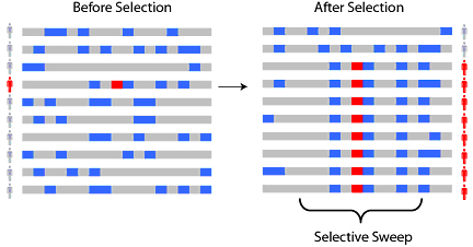
A new beneficial mutation arises in an individual (shown in red). It will rise in frequency in the population, leading to a characteristic reduction in diversity. Over time, genetic recombination and new mutations will build back the diversity, and the signal is lost.

Eventually, new mutations will creep in again, and generations of sexual reproduction would build back the diversity. However, if the loss of diversity was sudden enough (strong selection) and not too long ago, you can still detect it today. There are statistical tests (Fst, iHS, XP-EHH) that can formally detect if the reduction in diversity at a given region is sufficient to infer selection. Sabeti et al have a nice review paper that discusses the different methods available to detect selection using genomic data.

Our Results

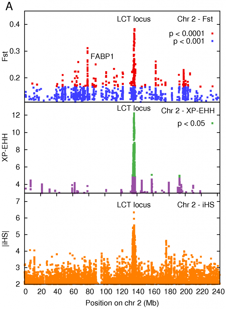
We used three different methods to detect selection, and our top candidate regions under selection are considered significant by at least two of the methods.

The strongest signal of selection, detected by all 3 methods, was a region on Chromosome 2 containing the Lactase gene (LCT), responsible for breaking down the lactose present in milk. Mutations in a neighboring gene in the cluster, MCM6, are associated with the ability to digest lactose in adulthood.

The strongest signal of selection was a region on Chromosome 2 that contained the LCT gene producing lactase, the enzyme that breaks down the lactose in milk. Interestingly, the default state in all adult mammals is to stop producing lactase in adulthood – our ancestors were all ‘lactose intolerant’. This makes sense from an evolutionary point of view, it forces children to wean from milk, and frees up the mothers resources. It turns out that different sets of mutations arose that gave European and African pastoralists the ability to digest milk. Those of us whose ancestors weren’t pastoralists still have trouble digesting milk.

This is a classic example of a selective sweep – a mutation confers an advantage (the ability to digest milk), and then sweeps through a population like wildfire. This result has been previously described in European populations, and also in African populations (including the Maasai) by Sarah Tishkoff and collaborators. Given that the Maasai consume large amounts of milk, it is not surprising that we see a very strong signal at this locus. We sequenced DNA in this region to confirm this result and, sure enough, we found that one of the lactase persistence conferring mutations identified by Tishkoff was present in the HapMap Maasai samples.

Two of the tests for selection that we used require that you make comparisons with another population. We chose the Luhya of Kenya as a our reference population. Among all the protein-altering mutations present in the data, the one that showed the largest population difference between the Maasai and Luhya (as measured by Fst) sits in the gene for a fatty acid binding protein FABP1. This protein is expressed in the liver, and the variant that occurs at higher frequency in the Maasai is associated with a lowering of cholesterol levels in Northern German women (n = 826) and in French Canadian men consuming a high fat diet (n = 623). Furthermore, studies in mice fed a high fat, high cholesterol diet showed that deactivating the FABP1 protein leads to protection against obesity, and lower levels of triglycerides in the liver, when compared to normal mice on an identical diet. These results suggest that this protein plays a role in regulating lipid homeostasis, and its selection in the Maasai may be diet-related.

On Chromosome 7, two of the methods we used to detect selection identified a cluster of genes that fall in the Cytochrome P450 Subfamily 3A (CYP3A). This family of genes is involved in drug metabolism, in oxidizing fatty acids, and in synthesizing steroids from cholesterol.

What’s next?

Computational methods can only take you so far. We have identified genes in candidate regions undergoing positive natural selection in the Maasai, possibly arising due to their unusual diet. But the case for selection can only be definitively made with an experimental study targeted to address the role of these genes in maintaining cholesterol homeostasis. We’re hoping to collaborate with experimental biologists to take these hypotheses forward and investigate their role in the evolutionary history of the Maasai.

So head over to PLOS, check out the paper, and let us know what you think.

Update: Here’s another blog post that discusses the paper, focusing more on the mixed genetic makeup of the Maasai.

References:

Kshitij Wagh, Aatish Bhatia, Gabriela Alexe, Anupama Reddy, Vijay Ravikumar, Michael Seiler, Michael Boemo, Ming Yao, Lee Cronk, Asad Naqvi, Shridar Ganesan, Arnold J. Levine, Gyan Bhanot (2012). Lactase Persistence and Lipid Pathway Selection in the Maasai PLOS ONE, 7 (9) : 10.1371/journal.pone.0044751

If you’d like to read more about selective sweeps, you may enjoy my post Why moths lost their spots, and cats don’t like milk. Tales of evolution in our time.

Pancakes, served with a side of science

There are few pleasures in life that exceed the simple joy of devouring home-cooked pancakes on a Sunday afternoon. I’m not much of a cook, but brunch is by far my favorite meal. So I decided that it’s time to take matters into my own hands, and improve my pancake making skills. Oddly enough, the first job I ever had as a college freshman was as a breakfast chef in my dorm. Back then, I’d make pancakes from a box, using Aunt Jemima’s pancake mix. I’ve since realized that it’s not much harder to make pancakes from scratch, and it’s a whole lot more gratifying. The quest for the perfect pancake is something of a lifelong journey. But unlike other boring journeys, this one is delicious, and served with syrup. Mmmm.

So where do we begin? I favor buttermilk pancakes myself, for their light and fluffy texture. If you go online and look for recipes, you’ll find plenty that claim to be the BEST buttermilk pancakes. Are these recipes really all that different? What sets them apart? And what’s the essence of a truly excellent buttermilk pancake?

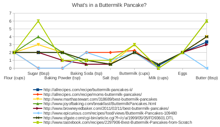
Like any scientist worth their salt (sorry), I decided to answer this question with a graph. After all, the whole is just the interaction of its parts. So let’s take apart what the web thinks of as the perfect pancake.

Above, I plotted the ingredients that go into a buttermilk pancake, according to eight highly rated online recipes. I normalized the recipes so that they all have the same amount of flour. You’ll see that there are certain essentials that you just don’t mess with. You definitely need one egg for every cup of flour. And there isn’t much variation in how much salt or baking soda you put in. On the other hand, these recipes vary widely in how much butter or sugar they include. Presumably, the excellence of a pancake is less sensitive to variations in these other ingredients. But which recipe do you follow? What’s a good empiricist to do?

Continue reading Pancakes, served with a side of science

I’m Top Quark, yo!

I’m thrilled to learn that I won the first prize in the 3QuarksDaily Science Prize, for my post on Crayola-fication of the World: How we gave colors names, and it messed with our brains. I’m pasting below the ‘acceptance comment’ that I left at the site.

WOW! I was woken up at 4:30 am by a very excited dad telling me that I’m Top Quark. It took me a good minute to parse what on Earth he was on about.

Thank you for your selection, Sean, and to Abbas and the rest of the 3QD gang for running the show. I’m particularly thrilled to be picked by Sean, as I’ve been a fan of his writings from back in 2004. In fact Preposterous Universe was the first science blog I came across, and to a voraciously geeky physics undergrad in a liberal arts college, it hit all the right buttons. I believe it was through Sean’s blog that I came across 3QD, another favorite over the years. So it means a whole lot to me to have made it here.

I also wanted to re-iterate Sean’s comments about the necessarily subjective aspects to prizes such as these. One of my favorite posts from the semi-finalists, by Christie Wilcox, didn’t make it to the finalists round, and the list of other finalists made for a seriously top notch reading list. It’s an honor to be listed among such high caliber writing. It’s all the more impressive when you realize how much time and effort bloggers put in to this, most of which is happening at the expense of sleep and other commitments. I’m thankful to 3QD for recognizing these efforts, and to the incredible readers who nominated and voted for these posts.

Here is what my dear mother suggests that I do with the prize money: “Aatish, put it in your bank in a trust, don’t blow it up. Maybe you should buy a new car. Can you buy a new car with $1000? Buy a Volkswagen. You have to claim it within 3 months. Do not be lazy about it.”

Thanks also to Sughra for designing the trophy logo, which I’ll put up with pride. 🙂

Sean Carroll has written an excellent short essay justifying his choices, highlighting the aspects of blogging that he sought out. I’m quoting from it below, you should read it in entirety here.

There is no simple and objective standard for what makes a blog post “the best.” “Blog is software,” as Bora Zivkovic likes to remind us — blogging is a medium, not a genre. Successful blog posts can be one word or ten thousand; a personal reflection or a rigorous analysis; an original idea or an insightful commentary; a devastating take-down or an inspirational message. But within these flexible parameter, there are certain aspects of blogging that make it special, and I looked for posts that took advantage of those unique capabilities. I wanted to choose posts that would be hard to imagine finding in any other medium, but whose quality measured up to the best of journalism or science writing. One frustrating aspect of a contest like this is that the prize is given to posts, rather than to blogs — for many of the most successful blogs, their charm comes from the accumulated effect of reading many posts over a long period of time. But okay, enough with the throat-clearing.

Without further ado:

First place this year goes to Empirical Zeal, for “The crayola-fication of the world: How we gave colors names, and it messed with our brains.” With many different criteria in mind, this post by Aatish Bhatia stood out among the rest. It’s just about the perfect use of a blog. For one thing, it looks gorgeous: all those colorful images, each of which actually serves a purpose. The writing is playful and clever; once you see the mantis shrimp telling you “DEAR MORTAL, YOUR RAINBOW IS PUNY,” you’re not likely to forget it. And most of all, the science is fascinating and important. To a physicist, there is a continuum of colors; but to our eyes and brains, “rainbows have seams,” and that affects how we think about the world. A completely deserving winner. (And don’t forget that there is a Part II.)

The 3 Quarks Daily Science Prize Finalists

Wow! I made it to the final round of the 3 Quarks Daily Science Prize. It’s an honor to be included among these seriously talented science writers. The final winners will be announced by Sean Carroll in a week.

Here’s the list of the other finalists, who you should definitely check out. I absolutely love this reading list.

To everyone who voted, tweeted and shared my article, thanks for all the crayon love. I’m very grateful for the overwhelming show of support. The color series are by far my most popular posts, and have spurred discussion on many online forums. Needless to say, I’m delighted!

Ready, set, VOTE!

And the nominees are..

The blog 3QuarksDaily is holding their annual Science Blogging competition. This year it’ll be judged by astrophysicist and all round science-superhero Sean Carroll. There are 107 blog posts competing, many of them quite excellent, a testament to the steadily growing talent pool in science writing. Your votes will decide the top 20 that make it to the next round.

Last year, back when I was a wee baby blog, I was incredibly honored that one of my early posts on blind cavefish made it to the final round. This time, I’m excited that two of my posts are in the running.

  1. What it feels like for a sperm describes the counter-intuitive science of fluid dynamics from the point of view of a sperm. It will be published in The Best Online Science Writing 2012 and arrive in bookstores in September.
  2. The Crayola-fication of the World is about the interplay between language, colors, and perception. It’s my most popular post and just passed a thousand(!) facebook likes today.

You can check out all the posts that are competing. Once you’re ready,

Head here to vote. Tell you friends to vote as well.

Spread the word, and support your friendly neighborhood science bloggers ;).